Money Management 101
Sun, Apr 9, 2017
by
MoneyTeamSP.cappertek.com
All of the information that is found below is from DrBobSports.com
Section 1: Primer
Tired of losing his money to the house, a bored millionaire in Las Vegas turns to you and offers you a proposition that you can’t refuse. He pulls out a stack of casino chips and declares:
“I’ve got a 100-sided, evenly weighted die, which I am going to roll. If it comes up 1 through 57 you win, if it comes 58 through 100 I win. We’re playing for even money. How much do you want to bet?”
How would you respond? Obviously you accept, but you are uncertain as to exactly how much you should wager – you are a solid favorite, but not an overwhelming one. The answer to this question is much deeper and more important to an investor’s bottom line than the average sports bettor ever realizes. This series of articles will provide the single most comprehensive investment optimization guide available on the internet, and will show you how to size your bets according to (1) your risk tolerance and financial goals and (2) the duration (number of bets) of your investment. Just as we use rigorous mathematical models to consistently pick winners against the spread, so too will we use simple but powerful financial formulas to achieve the greatest risk-adjusted return possible from those selections.
For bettors with a relatively low risk tolerance who are investing their money for one season, we will describe how to use a relatively flat betting structure, where your bets remain constant throughout the season, and how you can use the star system optimally. For bettors who are more risk tolerant, or who are investing over a period of several seasons (one sport over several years, or several different sports in one year), we will outline a more aggressive growth strategy with optimally fluctuating dynamic bet sizes.
For the bettor who just wants an approximation of what is generally correct, we will outline a summary in the next section. For the more advanced bettor who is curious to learn the fundamental logic behind our bet sizing systems, we will then describe the mathematics behind the Kelly Criterion, a formula which relates edge and odds to bet sizing for optimal investment in the sections that follow. We will continue to explain some of the nuanced concepts, such as simultaneous/sequential events, return/volatility ratios, and fractionalization. This should help illustrate how powerful the very simple, yet frequently misunderstood formula can be when applied correctly, and how to avoid disastrous mis-applications of growth sizing.
Section 2: Summary
When selecting the optimal investment, a bettor should seek a strategy that maximizes their utility. I aim for utility maximization, because depending on a bettor’s long-term financial goals, they can have very different marginal values for their money. Betting strategies can be aggressive or conservative, although in reality even my aggressive strategies are somewhat conservative compared with the ridiculous over betting advice that one will often find online. Strategies can also be either flat (where every unit is the same) or progressive (where units grow or decrease with the bankroll). For both flat and progressive strategies, bet sizing is correlated to confidence (more confidence = larger bets). Yet where other touts’ unit sizing is arbitrary, I size wagers as described by mathematically optimal ratios for growth as correlated with win percentage confidence. Furthermore, all necessary precautions have been taken to avoid over betting, the dangers of which are explained in Section 5.
1. Short Term Investment / Low Risk / High Probability of Positive Return
Short term investors who are seeking a safe, high probability return should bet 1% of their initial bankroll per star, resetting their bankroll size every year. Regardless of how well or poorly I perform in the short term week to week, these bettors should continue to bet 1% of their initial bankroll per star, and should not vary the bet sizes.
For example, in Week 1 Football I may have a 4-Star Best Bet, two 3-Star Bets and a 2-Star Bet and three Strong Opinions. On a $10,000 bankroll, the bettor should wager $400 on the 4-star, $300 on each 3-star and $200 on the 2-star, for a total of $1,200 wagered. Some bettors choose to treat Strong Opinions as 1-Star best bets. While my Strong Opinions have been 55% winners over the past 10 years, I consider them to be more volatile and less likely to win than my best bets. Betting Strong Opinions increases return, but also increases risk and volatility.
At the end of the season, the bettor should remove 100% of their profits, and then apply the same base initial bankroll for the start of the next season.
2. Short Term Investment / Moderate Risk / High Probability of Positive Return
These investors will follow the same model as Type 1 investors, but if they can afford to be more aggressive with their bankroll (i.e. their sports betting bankroll represents a lower portion of their overall net worth) then they can be less risk-averse, and bet 1.5% of their initial bankroll per star, and should not vary their bet sizes. This is approximately the optimal size for investing in my picks for a one to seven season period.
3. Long Term Investment / Low Risk / High Expected Return
Investors who want to achieve the greatest expected return need to have the capability to lock their money away for several seasons in a row, and ignore the month to month swings of Kelly Criterion investing. Progressive growth can be frustrating and counter-intuitive in the short run, and can be particularly frustrating during middling seasons. Kelly growth will outperform flat betting in the very long run by performing much better during very good seasons (winning a lot more) and very bad seasons (losing a lot less) while performing slightly worse in average, middle of the road seasons. Thus, the KC has a higher expected return, but a lower probability of positive returns. This is explained in greater detail in Section 7.
Before committing to a long-term Kelly growth strategy, readers must examine the rest of the articles which follow in order to fully understand the power as well as the dangers of long term growth. Since win-rates are never completely certain, we temper the Kelly Criterion with fractionalization and simultaneous event calculators. Lower risk, long term investors would be advised to use Kelly sizing of around 33% to 40% of a full Kelly Unit.
Again, I cannot stress enough the importance of thoroughly understanding the Kelly Criterion before committing to it.
4. Long Term Investment / Moderate Risk / High Expected Return
Investors who truly understand the Kelly Criterion and are willing to take a higher risk / very high expected return approach can apply 50-60% Kelly growth.
Section 3: Kelly Criterion
Much of the following section will likely be familiar territory to readers who have spent time in private equity or as a part of a hedge fund, as the principals of optimal investment and growth are very similar in sports betting. Just like a portfolio of stocks, the long-term sports bettor has one goal: to capture the greatest long term risk adjusted reward.
The first step towards accomplishing this goal is to utilize the Kelly Criterion (KC). The mathematics behind the KC were first alluded to by Daniel Bernoulli in the early 1700’s, and were later separately explained and applied to finance and gambling by John Kelly Jr. in 1956. Like most brilliant formulas, the KC is simple: it states that when one is presented with an opportunity to invest in a series of positive expectation wagers, whether they are Dr. Bob’s sports bets, a card counter’s blackjack hands, a hustler’s unfair coin flips or dice rolls, a guru’s stock prices, or anything else, using the KC to determine the percentage of one’s bankroll to invest in each wager will result in the greatest long term growth.
The KC maximizes long term growth by finding the optimal percentage of a bankroll that should be invested which will cause the greatest expectation of the logarithm of the outcomes. Described less cryptically, this means that the single greatest expected growth can be achieved by investing the portion of your bankroll defined as (O*w-l)/O, where O are the odds received, w is the probability of winning and l is the probability of losing (1-w).
For example, consider the millionaire’s coin from the Primer, which will come up heads 57% of the time, and pays out even money. In this case, your odds are 1:1, your w is .57 and your l is .43, so the bettor should wager (1*.57-.43)/1 is .14 or 14% of your bankroll. Thus, the KC dictates that you should continuously invest 14% of your current bankroll on the next flip. Whether you have won or lost several in a row, if you keep investing 14% of your current bank roll on the next flip, you will grow your initial bankroll at an optimum (unbeatable) rate.
If you are rolling a fair die but are getting paid 10:1 when the side you pick comes up (instead of 5:1) then your KC would be calculated as ((10*.1666-.8333)/10) or 8.33%. Optimal Kelly growth dictates that you would wager 8.33% of your current bankroll per roll of the die.
In sports betting, we are typically getting laid 10:11 odds, so we have to bet 11 to win 10. If we know the likelihood of a particular team covering the spread, we can decide exactly what the optimum bet size is. If we have a 55% chance of winning, then we should invest ((.909*.55-.45)/.909) or 5.5% of our bankroll. If we are particularly certain about a game, and estimate a 59% win probability, then we should invest ((.909*.59-.41)/.909) or 13.9% of our bankroll.
Before we continue, note that these examples and the following simulation make two major assumptions: (1) that we can quantify our edge exactly, and (2) that the events take place sequentially. In real life, it is very difficult to perfectly quantify our edge, and we must often bet on several events at once (a week or a particular time block of games), and therefore the KC requires much modification from its pure form. These issues are discussed in Sections 5 and 6, but for now we continue on with a ‘perfect world’ (where all information is known and all events are sequential) simulation.
Section 4: KC Simulation
To demonstrate this power visually, consider the following graphs where two bettors pursue different investment methods while picking the exact same sides of games. Each bettor starts with $100 and wins 55% of his games, and gets paid 10:11 odds when he wins. The first bettor (blue line) bets exactly $5.5 per game forever, while the second bettor (red line) utilizes the Kelly criterion and bets 5.505% of his bankroll, decreasing his bet size after losses and increasing it after wins. To create these graphs, we used a random number generator to determine whether a particular game that both bettors were wagering on was a win or a loss.
Through 50 bets
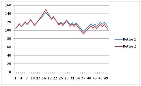
Bettor 1: 108 Bettor 2: 102
In the extremely short term, there is little difference between an investor using the KC and the flat bettor. When a bettors’ short term record is very good or very bad, the KC will outperform the straight bets, while records near .500 will slightly favor straight betting.
Through 150 bets
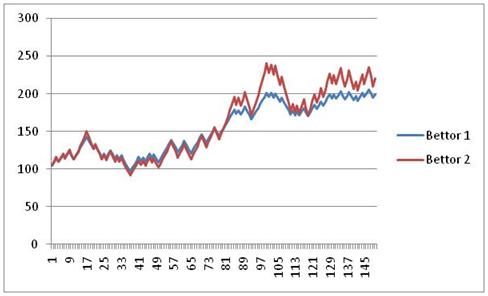
Bettor 1: 199 Bettor 2: 220
Still in the short term, you can see how the KC bets move drastically away from the flat bets on good runs, but falls quickly on bad runs. However, as they swing up and down, the KC bets slowly separate themselves.
Through 400 bets
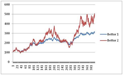
Bettor 1: 316 Bettor 2: 460
As we begin to amass a reasonable sample size, we can see the Kelly bettor beginning to pull away. With a bankroll of $460, the Kelly bettor will wager $25.32 on his next game, while the straight bettor is still betting $5.5 per game.
Through 1000 bets
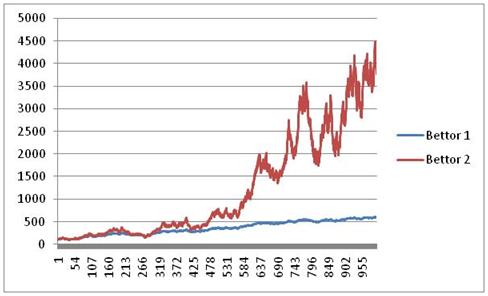
Bettor 1: 608 Bettor 2: 4,148
As we move into 1000 sequential bets, the Kelly bettor with his optimally increasing bet size crushes the straight bettor. At 1000 bets, the straight bettor is still betting the same $5.5 per game that he was at the beginning of the season, while the Kelly bettor will bet $228.34 on his next game. Notice that though the KC bettor is crushing the flat bettor, he also must endure several up and down swings of more than $1000. In fairness, this is also a fairly tame sample, although it was not engineered to be so and rather was just the product of a random number generator. Other samples have even more radical swings than this one, crashing up and down violently in pursuit of the overall upward trend.
Also, keep in mind how stressful these swings of Kelly Betting can be. Around bet #740, the Kelly bettor hits $3500. He then goes on a massive downswing over his next 100 bets (think: an entire football season) and loses half of his bankroll! It’s not until after his 900th bet that he again crosses $3500. Then, over the next 50 or so bets, he swings up to $4000, down to $2800, up to $4500, and so forth. While growth is being optimized by full Kelly wagers, a bettor who cannot keep his eye in the long term may find the swings too unpleasant to handle… especially in a scenario where you don’t know beyond all doubt that you have a long term edge.
Through 3000 bets
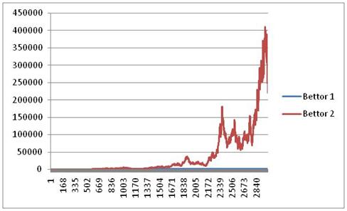
Bettor 1: 1,279 Bettor 2: 219,530
Over 3000 bets, the tremendous advantage of Kelly betting becomes even clearer. The Kelly bettor has run his bankroll to $219,530, while the straight bettor is at only $1,279. Again, notice the drop from $400k to $200k over the last few bets to close out the season.
Through 75000 bets
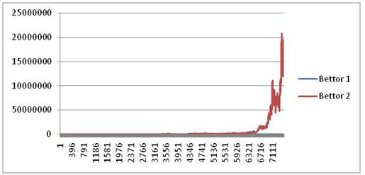
Bettor 1: 2,571 Bettor 2: 185,749,278
The final example is more of an academic exercise to drive the concept of Kelly betting home – after 7,500 bets the straight bettor has increased his initial $100 to a respectable $2,571… but the Kelly bettor has run his initial $100 to an astounding $185 million. This exercise serves to illustrate the tremendous advantage created by compounding bet sizes to grow one’s bankroll.
In addition providing for optimal growth, the Kelly Criterion also never allows the bankroll to drop to zero. Even if the bettor experiences terrible luck and loses a long string of games in a row despite being on the correct side, they cannot go broke, as they will have wagered increasingly low amounts as they ride their cold streak. In the long run, any positive expectation wager bet according to the Kelly Criterion will grow to infinity, continually increasing by ever larger amounts -and no matter how bad it runs for a period of time, it can never, ever hit zero.
Those who do not fully understand the nuances and implications of the Kelly Criterion often regard it as either mystical mathematical voodoo beyond the realm of common understanding, or as a misguided gambler’s foolhardy get rich quick scheme. In reality, it is just a valuable and underutilized tool for people who are consistently making positive expectation picks over the very long term, and is useful for maximizing expected growth while controlling the volatility to growth ratio. In the presence of uncertain information (i.e. true win percentages), Kelly betting should be tempered or fractionalized. Further explanation, examples and discussion of the Kelly Criterion are provided in the following sections.
Section 5: The Dangers of Over-betting and Over-Estimating your Edge
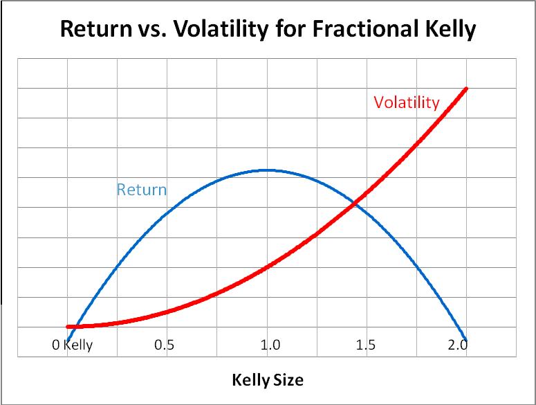
These graphs illustrate the long term power of using Kelly sizing to increase one’s bankroll over time, and beg the question, ‘if Kelly betting will lead to such incredible returns, then betting double or triple Kelly must lead to even higher returns!’ Referred to as ‘over betting,’ this misguided notion is one of the reasons that so many +EV sports bettors go broke just like their square compatriots. It turns out that someone betting 1.5 Kelly has the same expected growth as someone betting 0.5 Kelly, but with tremendously wilder upswings and downswings, and much more risk. Betting 2 Kelly actually has the same expected return as not betting at all: exactly zero, and betting more than two Kelly has a negative long term expected growth even if you are making positive expected value bets, and your bankroll will eventually fall to zero! In conclusion, Kelly sizing is in fact, as has been stated several times, the point at which return is exactly optimal.
Another important point to consider is that the dangers of over-estimating and over-betting your edge are not restricted to Kelly Betting. Flat bettors or even bettors who gamble ‘however much they feel like’ on a given trip to the casino frequently over-estimate and over-bet as well. Generally, bettors this unsophisticated are over-betting no matter what they do; they have zero edge at best, and probably a negative edge expectation, and shouldn’t even be betting in the first place. Yet, many advantageous cappers or bettors who buy my picks can unwittingly over-bet as well.
In addition to the dangers of over betting, the Kelly Criterion also has large swings compared to flat betting. For example, a given positive expectation wager that compounds at 10% per time unit will eventually double, and of course grow to infinity. However, since the swings with Kelly betting are so large, the initial bankroll actually has a 1/3 chance of being cut to half its initial value at some point before doubling. To an academic, this is immaterial, since they can keep their eyes on the long run expected growth. However, to investors who are often investing money for a shorter period of time and expecting immediate and consistent returns, this relatively high short term risk and volatility is unacceptable.
However, because variance is exponentially related to return, we find that cutting the bet size in half causes only a nominal reduction in expected growth, but square roots the variance. In other words, if we were to bet one half Kelly unit on our 10% per time unit (with full Kelly) proposition, we would grow our funds at a slightly slower rate of 7.5% per time unit while our risk/variance/volatility would be the square root of what it was previously. To use the previous example, we would now fall to 50% of our starting bankroll only 1/9 (rather than 1/3) of the time before doubling it – a much more tolerable level of risk for the average investor.
Betting one half Kelly unit instead of a full unit also helps prevent accidental over betting when we may have overestimated our edge, and we have already examined how destructive this can be. For example, if a bettor estimates his win percentage to be 58%, he would accordingly bet 11.8% (at 10:11) of his bankroll following full Kelly sizing. But, suppose that despite correctly picking a winner, the bettor had incorrectly assessed the real win percentage, and the side he picked would in fact be a winner only 55%, rather than 58% of the time. In this case, he should have bet only 5.5% of his bankroll, and since he overestimated his edge by 3% he actually over bet and wagered more than 2.1 Kelly. This will result in a negative expected growth despite the fact that the bet was still positive expected value, and would win 55% of the time. However, if the bettor instead followed a policy of betting ½ Kelly, overestimating win percentages is not nearly so dangerous. In this case, the win percentage miscalculation would have caused him to mistakenly bet twice the determined appropriate bet size… and he would have bet 1.0 Kelly instead of ½ Kelly, causing himself no harm whatsoever.
Full Kelly wagering is optimal when you know the odds exactly (as might a card counter who is aware of precisely which cards remain), but is too dangerous when positive expectation wagers are less certain. Bettors are well advised to halve or even third their bet sizes to cut down immensely on volatility while sacrificing relatively little expected growth.
Talk to any career bookie, and you will find a shocking truth: many (maybe even as high as 20% or 30%) sports bettors actually win over 50% of their games in the long run. However, their concepts of money management are so poor that almost all of them over bet wildly, driving their long term expectation to zero, and they all end up completely broke. The following anecdote, which could be any one of a million different bettors, illustrates the dangers of over betting:
“This guy Archie came into my book on the first week of September and bet about $1k on ten different NFL games. He ended up going 9-1, and turned his $10k into $18k. (n.b. we are ignoring vig for the sake of simple calculations) I knew he would be back though, and sure enough he was there the following week, betting $2k on nine different NFL games and totals. He got hot again, and went 7-2, and his $10k had now grown to $28k in just two weeks. I wasn’t worried though, because the story is always the same with these guys. In week three, he came in with 7 more ‘locks’ and put $4k on each game, only to go 1-6, losing three of the games in the last minute. Frustrated with his bad luck, he put all of his remaining $8k on the Monday Night Under, which busted when the Broncos scored a meaningless touchdown in the final minute. Three weeks after he started, Archie was broke.”
Archie is a prototypical gambler with absolutely no investment discipline. He started out with $10k, went 17-10 (63%) and ended up broke. Rampant over betting is a great way to empty your pockets while winning two thirds of your games. If Archie had just flat bet $500 per game the whole way through, he would’ve turned his $10k into $13.5k in three weeks. If he had bet 5% of his bankroll on each sequential game, he would have run his $10k up to $18.7k, and then slid in week 3 to finish at $13.7k, netting a $3.7k profit, albeit with some big swings. Does this story sound familiar? It should – it describes about 90% of the gamblers you’ll find at any given time in a Las Vegas sportsbook.
Section 6: The (Very Dangerous) Difference between Simultaneous and Sequential Events
An astute reader will observe that thus far all discussion of the Kelly Criterion has relied on events occurring sequentially. In the real world, bettors usually bet on a whole weekend’s worth of games at once. At best, they can bet on them a few at a time (time slot clusters), but they can never bet sequentially, adjusting their bankroll one game after the other. It would be a huge mistake to bet on simultaneous games as if they were sequential. In fact, betting on enough events simultaneously might even violate the principle that the KC can never reduce a bankroll to zero – if one wagered on 20 simultaneous 55% events at the KC recommended 5.5% per event, it’s hypothetically possible that they could lose all 20 games, and go broke.
Fortunately, there are easy to use calculators available for simultaneous event Kelly bet sizing which examine the likelihood of each individual outcome, and then the probability distribution of wins and losses, and then optimize the exact investment percentage for a quarter, half or full Kelly bet.
Consider the case of 10 simultaneous events, five of which are 54% and five which are 56%. Were these events sequential, we would invest 3.39% per game at full Kelly on the first five wagers, and 7.60% per game on the second five. If these ten events occur simultaneously, we would wager only 1.91% per game on the first five and 4.66% per game on the second five, and in total we would have 32.85% of our bankroll riding on these ten simultaneous events. As we calculate wagers for more simultaneous events or for events with higher win probabilities, the amount invested on the entire group approaches, but never hits 100%, and thus as expected we can never go broke.
The growth of advantageous wagers on simultaneous events is obviously much slower, but is also much less prone to wild swings of variance. Failing to reduce bet size for simultaneous events, and treating wagers as if they were sequential will undoubtedly result in over betting, wild variance and negative expectation.
Section 7: Contrasting Flat Betting with Kelly Betting
By now, hopefully you have a basic understanding of the basic concepts that define optimal bet sizing. We are aiming for long term growth, a reduction of risk, and an intelligent relationship between sizes. We have discussed the Kelly Criterion as a principle for forming the basis of sizing, but have shown the various dangers relying on pure KC creates.
Furthermore, consider that using Kelly growth (versus flat betting) increases your expected value over a given sample, but also decreases your chances of being a net winner. Consider an extremely basic example where you bet on two consecutive games that you have a 55% chance of winning. Flat Bettor has $10,000 and wagers $500 per game, while Kelly Bettor has $10,000 and decides to bet 1/2 Kelly sized wagers, and bets 5% of his current bankroll per game. Here is the outcome distribution:
| Flat | ||
|---|---|---|
| 2-0 | 0.303 | $1,000.00 |
| 1-1 | 0.248 | $0.00 |
| 0-2 | 0.203 | -$1,000.00 |
| Net EV | 100.00 | |
| Win % | 0.303 | |
| Kelly | ||
| 2-0 | 0.303 | $1,025.00 |
| 1-1 | 0.248 | -$25.00 |
| 0-2 | 0.203 | -$975.00 |
| Net EV | 106.44 | |
| Win % | 0.303 | |
Notice that the Kelly Bettor does better on the extremes (wins $25 more when he goes 2-0, loses $25 less when he goes 0-2), and that the flat bettor does better in the middle (breaks even at 1-1, while the Kelly bettor loses $25). The math behind the Kelly Bettor losing despite going 1-1 is simple: $X * 1.05 (win) * 0.95 (loss) = 0.9975 $X.
Also note that although the Flat bettor wins more often, the Kelly Bettor has a slightly higher expected value. The Kelly bettor expects to win $106.44, while the flat bettor expects to win $100 from these bets. Therein, as they say, lies the rub – betting Kelly is more volatile and will cause you to win less frequently, but you will perform much better on both extremes, and have a slightly higher EV.
Consider the same scenario, over 5 bets:
| Flat | ||
|---|---|---|
| 5-0 | 0.050 | $2,500.00 |
| 4-1 | 0.206 | $1,500.00 |
| 3-2 | 0.337 | $500.00 |
| 2-3 | 0.276 | -$500.00 |
| 1-4 | 0.113 | -$1,500.00 |
| 0-5 | 0.018 | -$2,500.00 |
| Net EV | 250.00 | |
| Win % | 0.593 | |
| Kelly | ||
| 5-0 | 0.050 | $2,762.82 |
| 4-1 | 0.206 | $1,547.31 |
| 3-2 | 0.337 | $447.57 |
| 2-3 | 0.276 | -$547.44 |
| 1-4 | 0.113 | -$1,447.68 |
| 0-5 | 0.018 | -$2,262.19 |
| Net EV | 252.51 | |
| Win % | 0.593 | |
Once again, Kelly Betting has a higher EV ($252.51 compared to $250.00). Again, it does better at the extremes, winning $262 more when it goes 5-0 and $47 more when it goes 4-1, and losing $238 less when it goes 0-5 and losing $53 less when it goes 1-4. Flat betting performs better in the middle outcomes, winning $53 more at 3-2 and losing $47 less at 2-3. Thus, the risk/reward of Kelly becomes clearer. Exactly 61.3% of the time, over a five bet sample, flat betting would do better than Kelly betting. However, in the 38.7% of the time that Kelly betting does better, it does so by much larger margins (especially in the 6.8% of 5-0 and 0-5 outcomes).
Once the sample sizes grow larger, the differences become more pronounced. Kelly betting becomes more +EV, but the percentage of the time that it is better overall grows smaller. With a 21-20 record over a 41 game sample at $500 a game with no juice, a flat bettor is +$500, but a Kelly bettor is actually -$12 despite the winning record! But with an unusually good record of 30-11 over that same sample, the Kelly bettor is +$14,583 while the flat bettor is only +$9,500.
In conclusion, bettors who are more concerned with maximizing their win probability in a given season, especially considering that one season’s worth of games is a small enough sample that the extra EV from Kelly betting is quite small, would be well advised to pursue a very flat betting structure. Bettors who are intending to invest for a longer period of eight seasons or more might want to pursue progressive wagers at a fractional Kelly.
I'd like to thank the crew over at DrBobsports.com for all of this useful information...it has helped me tremendously and I am posting it here, to help all of you as well.